Linear Motion via Higher Dimensional Rotations

Expressing a known behavior in a new way has the potential to expose new thinking and opportunities.  I was thinking a bit about how to express absolute position exclusively via rotation.  I started to think about the rotating light in a light house and the light it would cast on a curtain hung between you and the light house and how the distance the light would appear to move across the sheet is not proportional to the angle of rotation of the light house; it would appear to decelerate until it is pointing at you before accelerating off.

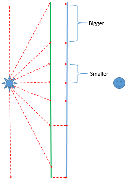
Clearly to maintain the proportionality of the angle of the lighthouse to the distance the light moves on the sheet, the sheet would need to be hung around the lighthouse:

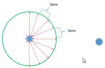
But if you hung the sheet like this, from your perspective as the observer, you would not see the light move proportional to the angle, in fact you would see it now accelerate until it faced you before decelerating away.

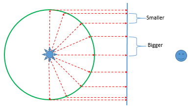
So what is the geometry of a curtain situated between you and the lighthouse such that the light would appear to travel across the surface of the curtain at a constant speed?  It would need to be some surface like this:

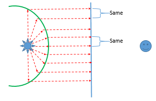
Below is a plot of the function that meets this requirement.  For convenience I turned this problem vertical such that the light house is situated at the origin, the curtain is the red curve draped around it from above and the angle is described as off of the vertical axis.

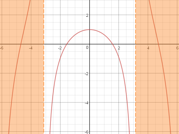
The formula for this curve is simply:

As you can see the horizontal range of this curve is from -Pi to +Pi and it’s beauty is that any angle off the vertical axis you strike the curtain at a point where it’s x coordinate is that angle; This relationship is ultimately the definition of this curve.  (This feels reminiscent of how the derivative of the function e^x is e^x and how this embodies what e is)

So with this function we can describe the position on a line using a rotation where the rotation is related in a linear fashion to the position.  Again, we do this by mapping the rotation to the curve and projecting the curve to a lower dimension (2d->1d).  We can simply scale the length of the line to any arbitrary distance we want it to represent.

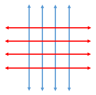
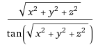
Now what I want to do is extend this up a dimension such that we can use a 3d source cast onto 2d surface warped in 3d space that can be projected down to describe position in a plane.  This has interesting parallels to cartography where the goal is to represent a position on a sphere on a flat map.  The surface and formula to accomplish this is the following:

*Sorry that is a little distorted due to the range… I don’t have a paid version of Mathematica and the free online one doesn’t recognize “PlotRange” option.

 

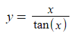
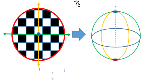
Now one thing to consider is how we define these angles when we get beyond a 2d rotation where there is simply a single angle.  One’s mind may jump to a spherical coordinate system but that route doesn’t get to our intent which is to describe linear motion via rotations.  This is because if you consider the rotations in a spherical coordinate system they would result in the following motions in the resultant projection we are interested in where one angle (polar angle) would result in motion in Blue and the other (radial angle) would result in the motion in Red.

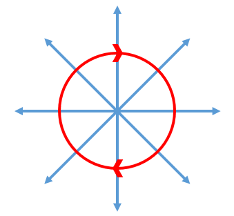
What we want is what is below where one angle is red and one is blue.

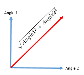
We accomplish this by considering each of the two angles independently and combining them as vectors to describe a single vector.  As you can see in the 3d formula I showed earlier this is the approach I use.

Now this can be hard to visualize so I really wanted to show what a sphere would look like that would project a checkerboard pattern into 2d but it proved awfully challenging to illustrate this, perhaps I’ll come back to another time.  This partially illustrates…

For future playing around, here is how this formula maps into spherical coordinates and then into cartesian coordinates:

• Polar Angle, P = Sqrt[x^2 + y^2]
• Radial Angle, R = ArcTan[y/x]
• Cartesian X =Sin[P]*Cos[R]
• Cartesian Y =Sin[P]*Sin[R]
• Cartesian Z =Cos[P]

Ultimately my secret goal all along here was to take this up yet one more dimension to a 4d surface.  I like to imagine this as having an etch-a-sketch control in front of me with three dials.  These three dials control the three angles in the 4d rotation to shine a narrow 4d beam of light at a 3d space warped in 4d space around the light source.  We would perceive that light projected into our 3d world as a small floating glowing orb where one of the three dials sends it left and right, one back and forth and the last up and down.

Here is the simple formula for that 3d surface bent in 4d space for that device:

Now what can we do with this?